Sunspots

• We have also used the sunspot data provided by the American Association of Variable Star Observers. (https://www.aavso.org/)
  • Data accessed through https://lasp.colorado.edu/lisird/

• Sunspots are temporary dark areas on the Sun's surface.
• They are caused by intense, concentrated magnetic fields that inhibit convection.

• Indicators of Solar Activity
  • High sunspot numbers are linked to more frequent solar flares and Coronal Mass Ejections.
  • Both release charged particles that disrupt our magnetosphere.
  • High sunspot activity raises the Sun's Total Solar Irradiance, which can influence Earth's climate and surface temperatures.hempelmann2012correlation

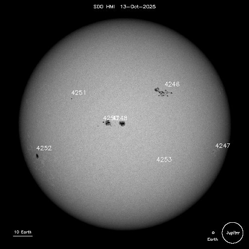Source: Solar and Heliospheric Observatory, NASA

Edit Distances

• Let \(P_1\) and \(P_2\) be two marked point processes: $$ P_1 = \{ (t_i, \vec{u}_i) \mid 1 \le i \le N_1 \} \quad\quad P_2 = \{ (s_j, \vec{v}_j) \mid 1 \le j \le N_2 \} $$
• The idea is to transform \(P_1\) into \(P_2\) using primitive operations, each incurring a cost.
• The primitive operations are:
  • Insertion: insert point \((s_j, \vec{v}_j)\) from \(P_2\) into \(P_1\), paying a cost of 1.
  • Deletion: remove point \((t_i, \vec{u}_i)\) from \(P_1\), paying a cost of 1.
  • Shifting: replace point \((t_i, \vec{u}_i)\) in \(P_1\) by the point \((s_j, \vec{v}_j)\) from \(P_2\), paying a cost of: $$ C\big((t_i, \vec{u}_i), (s_j, \vec{v}_j)\big) = \lambda_0 |t_i - s_j| + \sum_{k=1}^{d} \lambda_k \big| \vec{u}_i(k) - \vec{v}_j(k) \big| $$
• The \(\lambda_k\) are user-defined normalizing constants intended to ensure that the different marks have comparable orders of magnitude.
• The edit distance is defined as the lowest possible cost necessary to transform \(P_1\) into \(P_2\).

Radial Basis Functions

• We use these edit distances with Radial Basis Functions (RBFs) for performing the forecasting.
• Simply put, it finds a functional relation of the form: $$ \hat{y}(\vec{x}, \vec{w}) = w_0 + \sum_{i = 1}^{k} w_i \, \psi\big(d_H(\vec{x}, \vec{c}_i)\big) $$
• Where:
• $\vec{x}$: the point process (e.g., the set of earthquakes in a week) for which we want to make a prediction.
• $\vec{c}_i$: point processes taken from the training set, which will be compared with $\vec{x}$.
• We take $100$ randomly chosen instances $\vec{c}_i$ from the training set.
• $w_i$: adjustable parameters found by least squares.
• $\psi$: taken to be the Gaussian kernel, $\psi(x) = \exp(-x^{2} / \epsilon)$.

• We predict the logarithm of the number of earthquakes, $\log(N + 1)$, in a certain day.
• The predicted values of $\log(N + 1)$ are then correlated with the maximum magnitude by means of Gutenberg-Richter's law.stein2003introduction

Dynamical Systems: A Brief Introduction

• A dynamical system is simply a system whose state evolves over time according to a fixed rule.
• Core Components:
  • State: A snapshot of the system at a specific time (e.g., position and velocity of a pendulum).
  • State Space: The set of all possible states the system can be in.
  • Evolution Rule: A mathematical rule ($f$) that describes how the state $x$ changes over time. $x_{t+1} = f(x_t)$
• Common examples include planetary orbits, weather patterns, and population dynamics.

• Many useful tools in this field:
  • State-space reconstruction based on time series of observations
  • Prediction by nearest-neighbors
  • Tools to detect coupling between two systems
  • and a lot more

Example: Lorenz System

Example: Hénon Map

• Numerous dynamical systems could be involved in the earthquake generating process.
• One example are the convection flows within the Earth's mantle (Navier-Stokes equations).
• The figure below shows an exaggerated diagram.

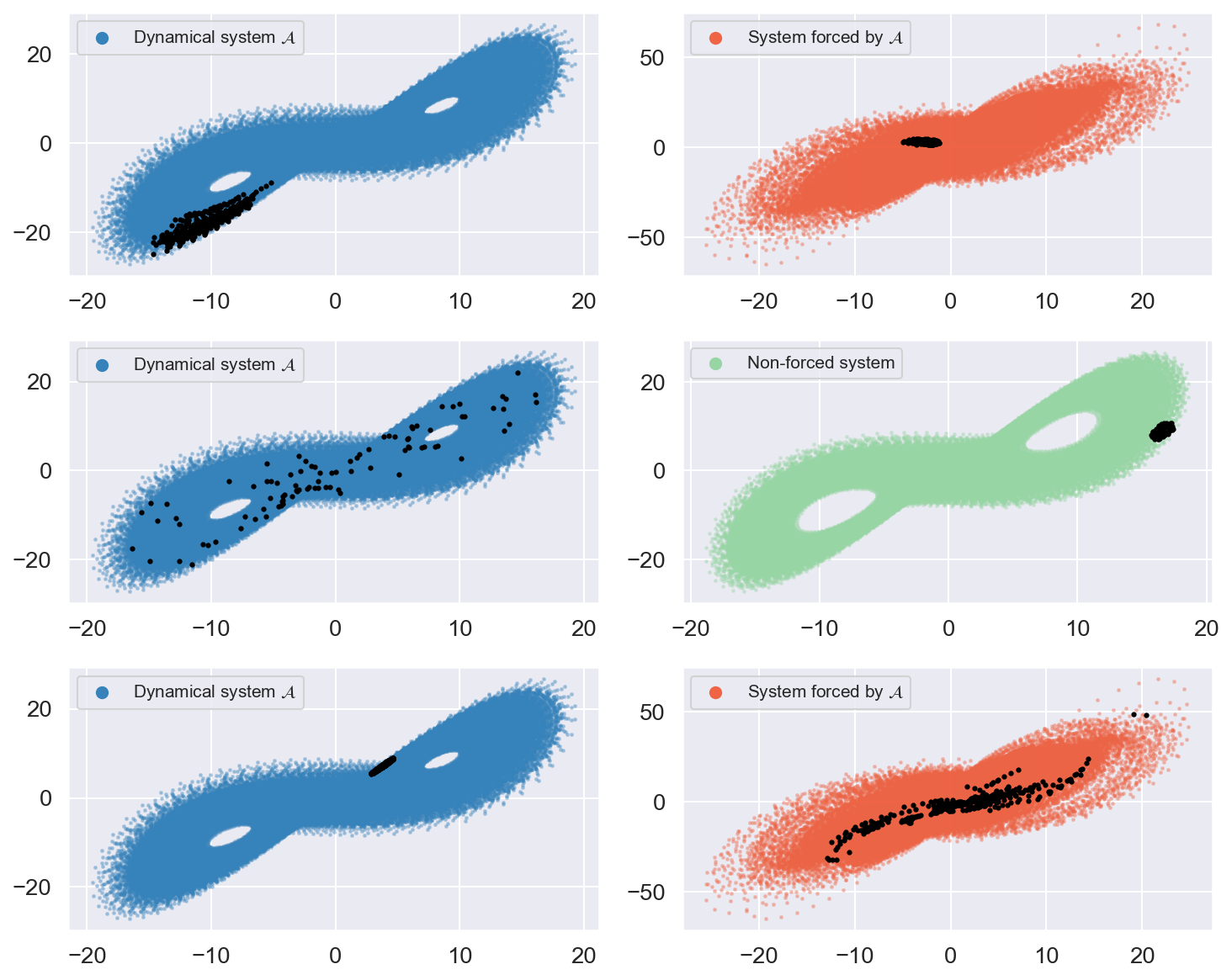
Coupling Detection Methods

• One dynamical system can have a strong influence in another (coupling).
• To measure coupling, we use two methods:
• Hirata et al. (2016)hirata2016plosone
• Andrzejak et al. (2011)andrzejak2011characterizing
• They both rely on the same basic idea:stark1999
• Measure systems $X$ and $Y$ at times $t_0$ and $t_1$, observing $s_X^{t_0}$, $s_X^{t_1}$, $s_Y^{t_0}$ and $s_Y^{t_1}$
• $s_Y^{t_0}$ and $s_Y^{t_1}$ are similar $\overset{\text{?}}{\Rightarrow}$ $s_X^{t_0}$ and $s_X^{t_1}$ are also similar
• Then we say system $X$ drives system $Y$

• Measure systems $X$ and $Y$ at times $t_0$ and $t_1$, observing $s_X^{t_0}$, $s_X^{t_1}$, $s_Y^{t_0}$ and $s_Y^{t_1}$
• $s_Y^{t_0}$ and $s_Y^{t_1}$ are similar $\overset{\text{?}}{\Rightarrow}$ $s_X^{t_0}$ and $s_X^{t_1}$ are also similar
• Then we say system $X$ drives system $Y$

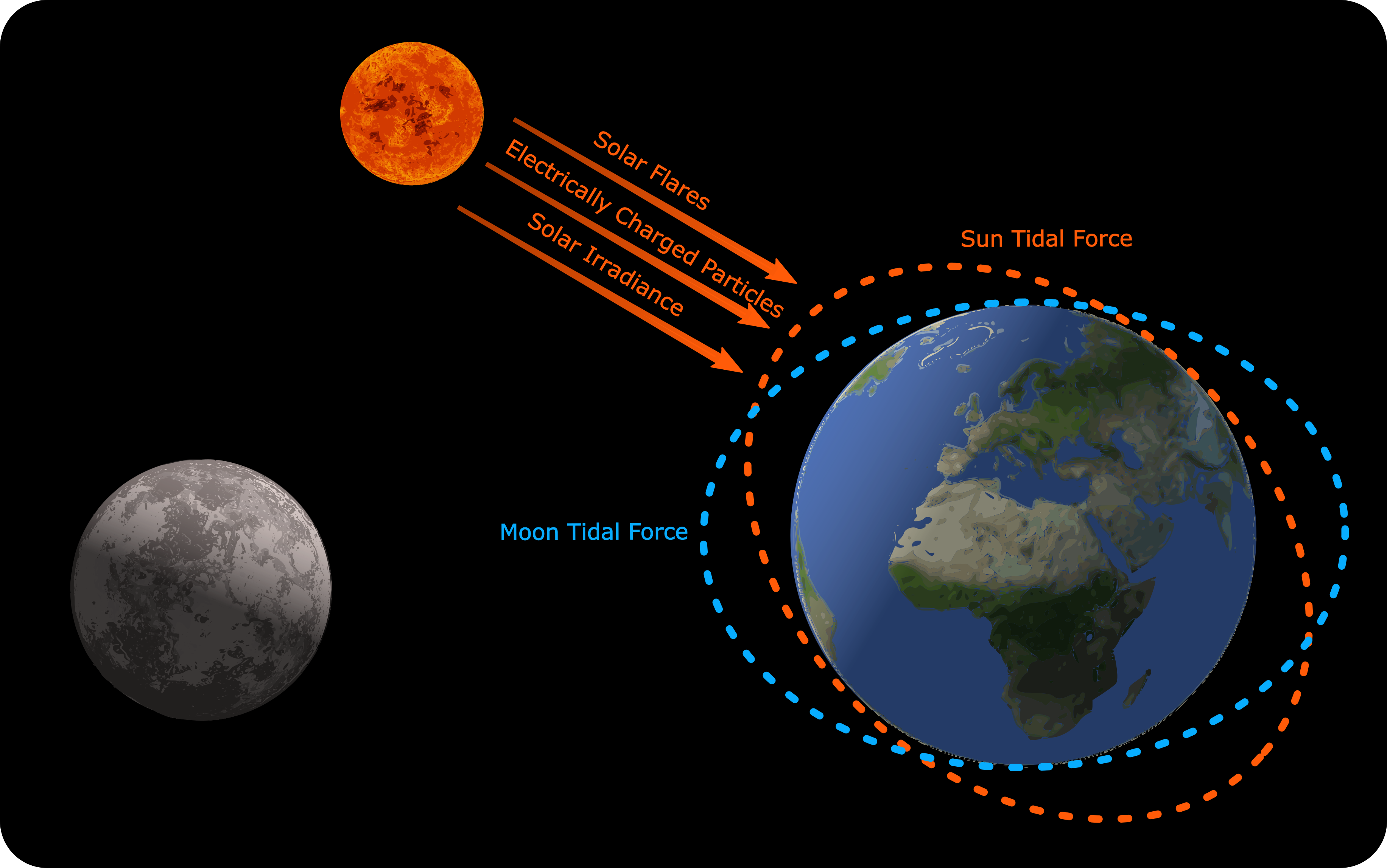
Effects of Lunar (and Solar) Tidal Forces

• The difficulty of earthquake forecasting is aggravated by the fact that:
  • we cannot yet enumerate all the external factors influencing earthquakes
  • or the degree of importance of each of these factors

• In the master's dissertation, the connection between Sun activity & earthquakes was analyzed.
• Here we continue investigating external factors that affect earthquakes
  • We began by analyzing tidal forces from the Moon
  • Solar tidal forces were analyzed, but were not as fruitful

• The influence of tidal forces has been investigated in the literature ide2016naturegeosciencehao2019evidence
• However, either:
• they analyze only correlation, without assessing its applicability in prediction;
• or they perform predictions for larger time frames (above 15 days)

• Tidal forces are theorized to influence earthquakes due to its ability to deform the continental crust
• This could play a significant role in the rate of elastic strain energy accumulation in faults
• Most importantly, it could be a significant agent that causes the initial crack (nucleation) that develops into an earthquake

• We simulated the trajectories of the Sun and Moon using the Python library Astropy.
• We calculated:
• hourly differential pulls on each region
• differential pull at the place and time of each earthquake in our catalogs

• To include sunspot and Moon tidal force data into our prediction framework, we modify our framework as follows:
$$ \hat{z}(\vec{x}, \vec{y}^{(1)}, \vec{y}^{(2)}, \vec{w}) = w_0 + \sum_{i = 1}^k \bigg[ w_i \, \psi\big( d_X(\vec{x}, \vec{c}_i) + \kappa_1 d_E(\vec{y}^{(1)}, \vec{y}^{(1)}_{\vec{c}_i}) + \kappa_2 d_E(\vec{y}^{(2)}, \vec{y}^{(2)}_{\vec{c}_i}) \big) \bigg], $$
• Where:
• $\vec{y}^{(1)}$: vector containing the 7 sunspot numbers referring to the same week as $\vec{x}$
• $\vec{y}^{(1)}_{\vec{c}_i}$: same as above, but referring to the same week as $\vec{c}_i$;
• $\vec{y}^{(2)}$: the $168$-dimensional vector containing the hourly tidal force collected over the 7-day window
• $d_E()$: the Euclidean distance

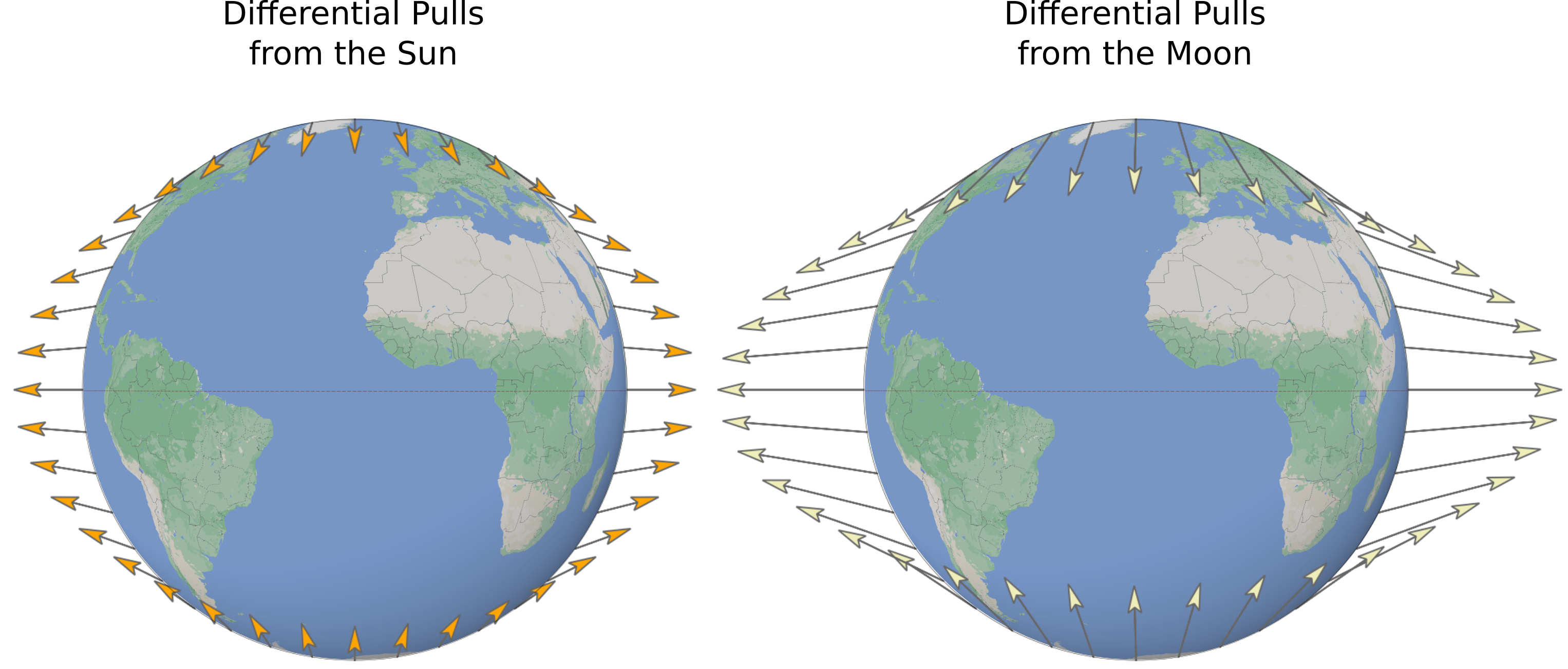
Tidal Force Calculation: Differential Pull

• What is commonly called tidal force is more accurately a differential pull.
• It arises because the Moon's gravitational pull has varying intensity across the Earth's diameter.
• The approximate differential pull on an object at the Earth's surface is given by:sawicki1999myths $$ \frac{2 G m_M r_E}{d_M^3} $$
• A similar effect occurs on both the near and far sides of the Earth.

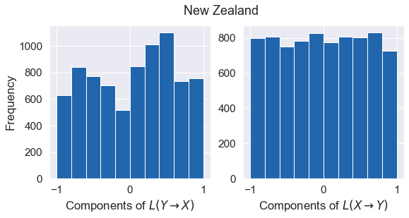
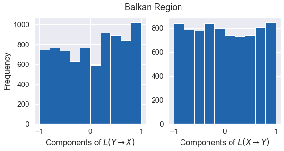
Causality: Andrzejak et al. Methodandrzejak2011characterizing

• Found evidence of Moon influencing earthquakes ($Y \rightarrow X$).
• Coupling measure $|L(Y \rightarrow X)| \gg |L(X \rightarrow Y)|$.
• Histograms for $L(Y \rightarrow X)$ (left) show irregular, slanted distributions, indicating coupling.
• Histograms for $L(X \rightarrow Y)$ (right) are nearly uniform, indicating no coupling.

Causality: Hirata et al. Methodhirata2016plosone

• Unidirectional coupling was also identified using this method.
• Generally, $p$-values for the Moon-to-earthquake ($Y \rightarrow X$) direction were much smaller than for the reverse direction.
• Exception: The Japan catalog, where the relation was inverted, possibly due to stochastic factors.
• Overall Conclusion: The collective results from both methods provide evidence for a causal coupling from the Moon to earthquakes.

Correlation: Tidal Force vs. Magnitude

• We also investigated the direct relationship between differential pull and earthquake magnitude.
• This analysis focuses on correlation to corroborate the causality findings.
• We calculated the average differential pull for earthquakes with magnitude $\ge m$, for various values of threshold $m$.

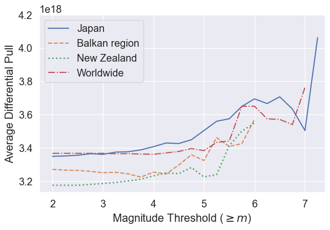
Correlation Findings

• Clear Trend: The average differential pull increases with the magnitude threshold across all catalogs.
• This indicates a tendency for larger-magnitude earthquakes to occur during periods of higher tidal force.
• Main Finding: A persistent positive correlation exists between lunar tidal force and earthquake magnitudes.

• We also compared the differential pulls of the 20% lowest magnitude earthquakes against those above various higher thresholds (e.g., >5, >5.5, >6).
• The earthquakes with larger magnitudes have larger differential pulls.
  • $p < 0.05$ for ~70% of the cases, with a Wilcoxon rank-sum test

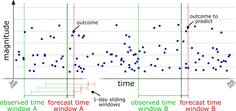
Improving Forecasting Accuracy

• Goal: Verify if Sun (sunspots) and Moon (differential pulls) data improve forecasting accuracy.
• Method:
  • Forecast the log-number of earthquakes: $\log(N+1)$.
  • This is then correlated with maximum magnitudes (Gutenberg-Richter law).

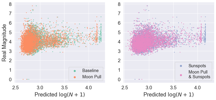
Example forecasts for New Zealand

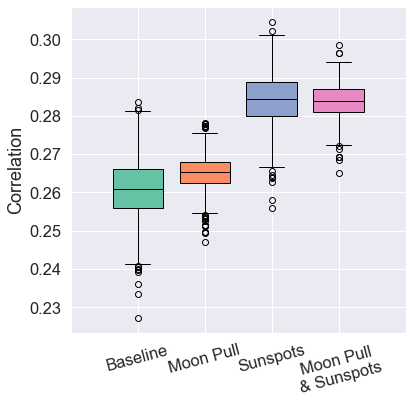
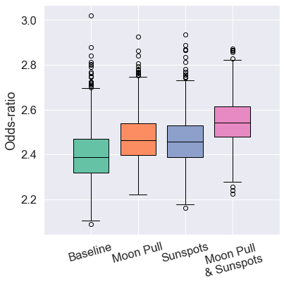
Forecasting Results: Japan

Japan (Nationwide)

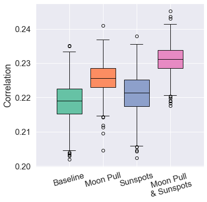
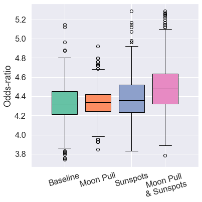
• Moon data slightly improves correlation.
• Best correlation gain (+5.37%) with Moon + Sun data.
• Odds-ratio only improves (+3.51%) when both are combined.

Touhoku Region

• Higher baseline accuracy.
• Significant accuracy gains.
• Correlation up to +29.62%.
• Odds-ratio up to +76.63%.

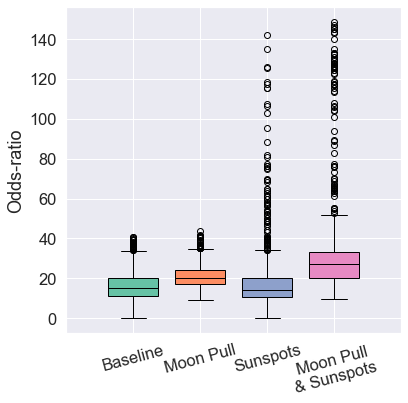
Forecasting Results: New Zealand & Balkan Region

New Zealand

• Sunspot data most relevant for correlation (+8.86%).
• Combined data yielded best odds-ratio (+5.72%).

Balkan Region

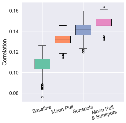
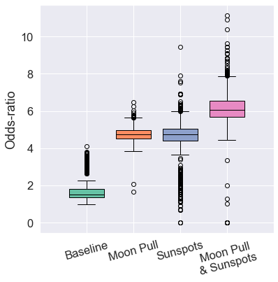
• Smaller subregion yielded higher correlations.
• Substantial increases in both metrics from Sun or Moon data.
• The highest accuracy is achieved when all data types were used simultaneously.

Conclusion: Summary of Findings

• Presented significant evidence that seismic activity is influenced by tidal forces from the Moon.
• Moon's Influence:
  • Established a unidirectional causal link (Moon's motion drives earthquakes).
  • Found a slight-to-moderate tendency for larger earthquakes to occur during periods of higher tidal force.
• Forecasting: Demonstrated that next-day magnitude forecasting accuracy improves when using lunar data, and even more so when combining lunar and sunspot information.

Pinpointing the Sun-Earthquake Mechanism

• Our previous work established a causal link: solar activity influences earthquakes.junqueira2022solar

• However, the physical mechanism behind this link is still an open question. Potential pathways include:
  • Interactions with the geomagnetic field
  • Emission of solar particles
  • Tidal forceside2016naturegeoscienceyabe2015tidal

• Our hypothesis: The thermal energy (heat) transfer from the Sun is a major player in driving changes in the Earth's surface temperature.
  • If it is a major player, then we can say it is being neglected in the literature.

Potential Mechanisms by Which Heat Could Affect Earthquakes

• Thermal Stress
  • Temperature variations can induce thermal stress in rocks, altering their mechanical properties and contributing to fracture kang2019review.
  • While surface heat penetration is slow, it can affect deeper layers over long timescales.kalogirou2004measurements
• Hydrological Cycle
  • Atmospheric temperature variations influence the hydrological cycle (evaporation, precipitation).
  • This impacts subsurface water flow and pore pressure within faults, potentially triggering earthquakes.wang2021earthquakes
  • Seasonal changes like snow/ice melting can alter pore pressure and load the Earth's crust.
  • Example: Fluid migration from snowfall may have triggered the M7.6 Noto, Japan earthquake in 2024.wang2024untangling

• Atmospheric Pressure
  • Changes in atmospheric pressure can induce small-scale clamping and unclamping of faults.liu2009slow
  • A recently identified phenomenon is "stormquakes", where intense storms generate seismic waves in the crust.fan2019stormquakes

• Thus, several plausible mechanisms have been proposed.
• However, the supporting evidence for these mechanisms remains largely inconclusive.
• This shows a clear need for further investigation into this area.

Seasonal Variation of Earthquake Location

• Analyzed the correlation between earthquake latitude and magnitude in the northern hemisphere, differentiated by season.
• A statistically significant lower correlation is observed during the winter ($p = 0.002$ via t-test).
• This indicates that larger earthquakes have a slight tendency to occur at higher latitudes during all seasons except for winter.

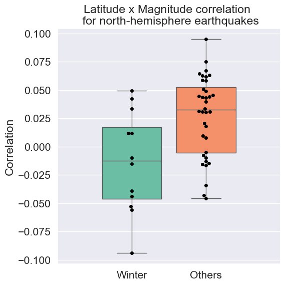
• This result points to a driving force connected to both latitudinal position and the cycle of meteorological seasons.
• Solar heat fits this description well, strengthening the hypothesis that it is a significant mechanism for the Sun's influence on earthquakes.

Are Solar Activity & Earthquakes Deterministic or Stochastic?

• We employed recurrence plots to test whether the time series are deterministic or stochastic.
• Methodology from Hirata, Y. (2021)hirata2021recurrence was used to count the variety of recurrence triangles.
• The method indicates that both solar activity and earthquake occurrences are stochastic.
• We conjecture that a portion of the stochasticity in seismic activity is inherited from the Sun

Illustration of a recurrence plot and recurrence triangles.

Super-exponential growth of recurrence triangle varieties for sunspots and earthquakes.

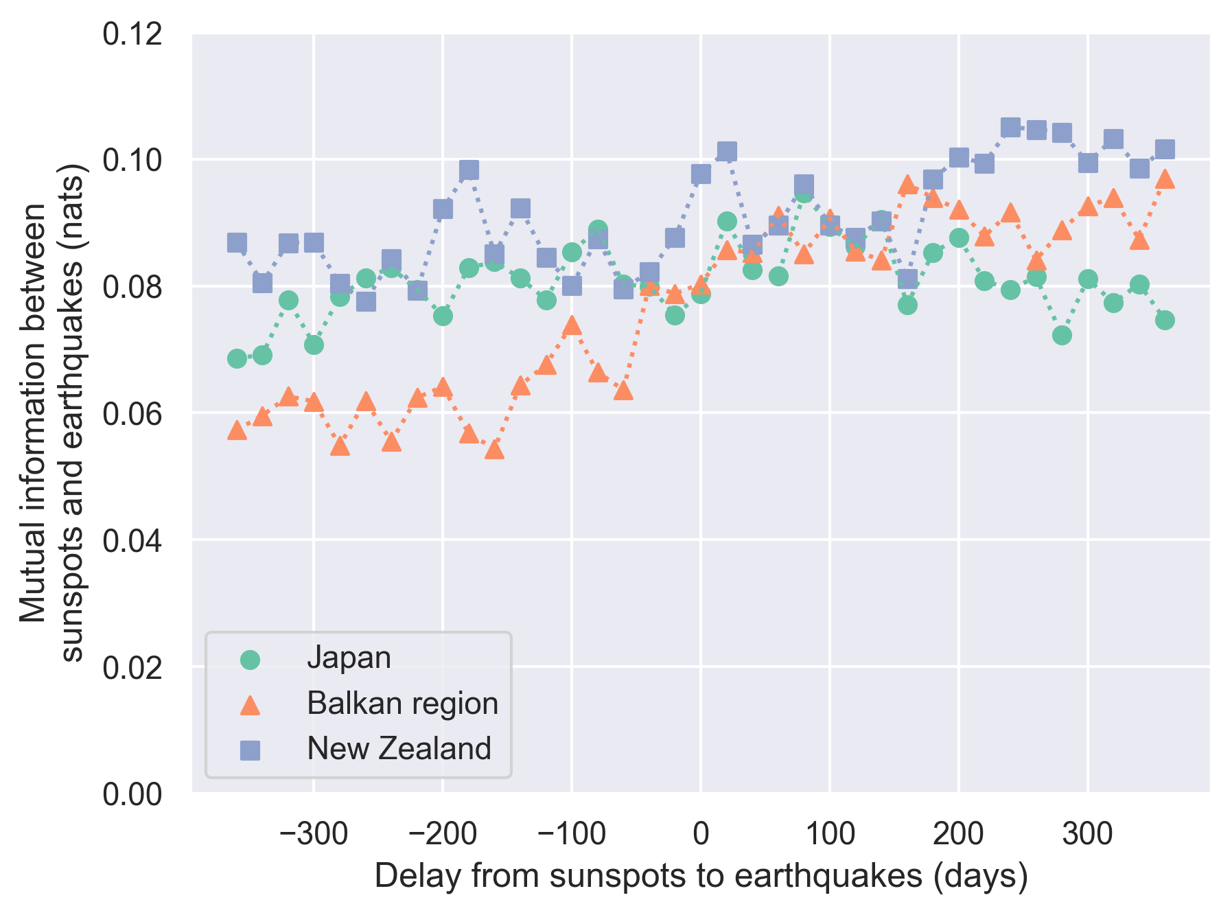
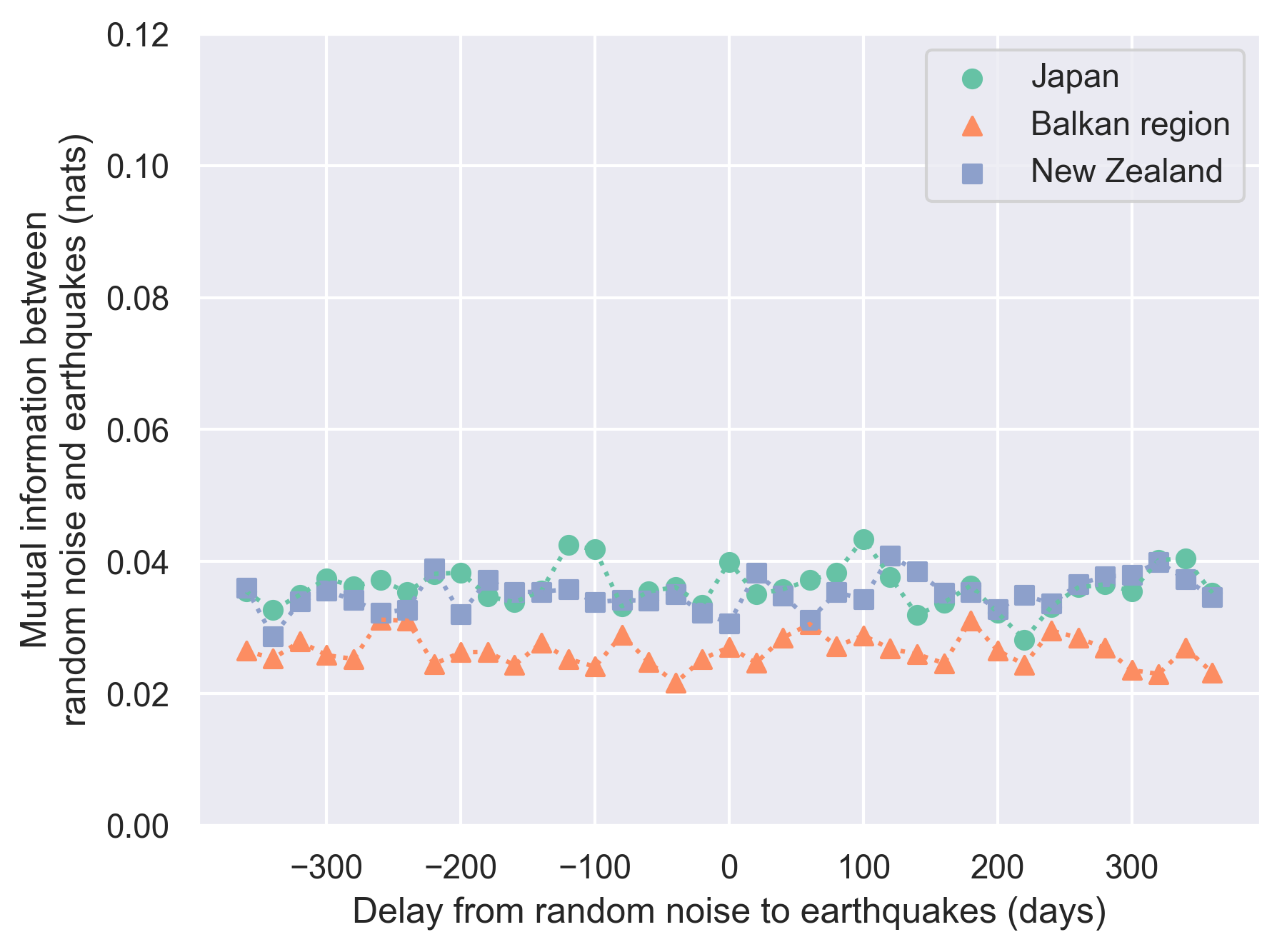
Mutual Information Confirms Shared Stochasticity

• Mutual information was used to quantify the statistical dependency (linear and non-linear) between the two systems.
$$ I(X; Y) = \sum_{x \in X} \sum_{y \in Y} p(x, y) \log \left( \frac{p(x, y)}{p(x)p(y)} \right) $$
• Mutual information is non-zero and significantly larger than that calculated with random noise.
• This demonstrates that information is shared between the two systems, reinforcing the previous conjecture.

The Sun-Earthquake Time Lag

• A key aspect of the Sun-earthquake relationship is the time lag between cause and effect, which has been largely overlooked in the literature.
• Mechanisms for solar influence require significant time to manifest.
  • e.g. Thermal energy from the Sun may take weeks or months to accumulate and impact secondary processes (e.g., ice melting, atmospheric pressure changes).pan2023annualseneviratne2010investigating
• Research Question: What is the time lag between changes in solar activity and their subsequent effects on Earth's seismicity?

• Used daily sunspot numbers with various time lags to forecast maximum earthquake magnitudes.
• The plots show how forecasting accuracy changes when sunspot data is time-lagged.

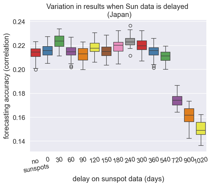
• Lags that offer statistically significant improvements (Bonferroni corrected $p < 0.05$):
  • Japan: 30, 120, 180, 240, 300 days
  • Greece: 30, 90, 120, 150, 180, 300 days
  • New Zealand: 60, 90, 120, 150, 180, 300, (...) days
• A delay of 120 days is the first significant lag common to all three regions, possibly related to seasonal changes.

• Recall that the mutual information for a zero-day lag was substantially lower than the peak values observed at non-zero lags.
• This further supports the existence of a delayed cause-effect relationship.

• Thus, in summary:
• A time lag exists between changes in solar activity and their effects on terrestrial seismic activity.
• A single, universal value for this delay does not exist; it is region-specific.
• The existence of a range of effective delays is physically plausible due to the multiple mechanisms by which thermal energy can trigger earthquakes (e.g., ice melt).

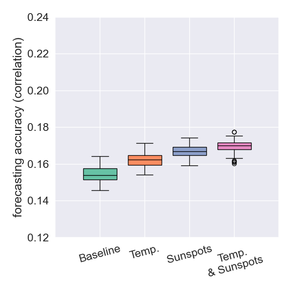
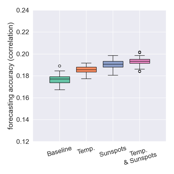
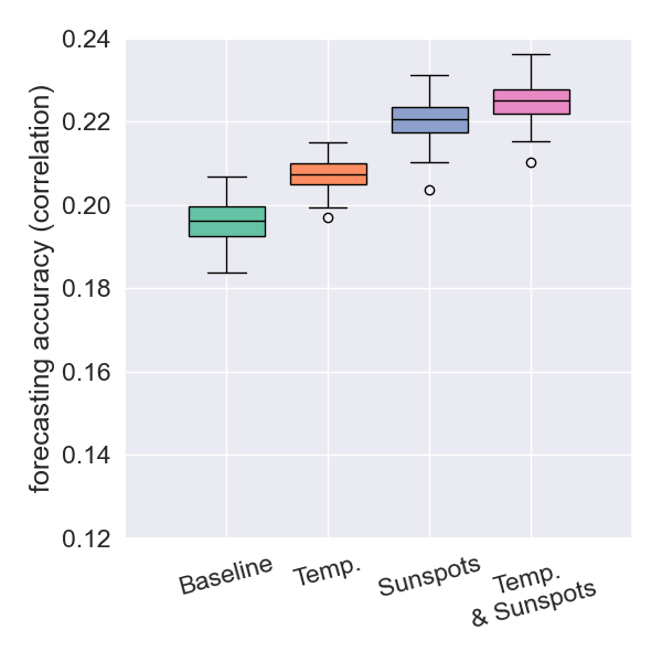
Forecasting With Surface Temperatures: Japan

• Data on daily average air temperatures from Tokyo, Stylida, and Wellington can, in most cases, improve the prediction of next-day maximum earthquake magnitudes.
• The results clearly indicate that incorporating surface temperature data helps to improve prediction accuracy.
• Combining both sunspot and temperature data achieved the highest correlation among all settings tested for this region.

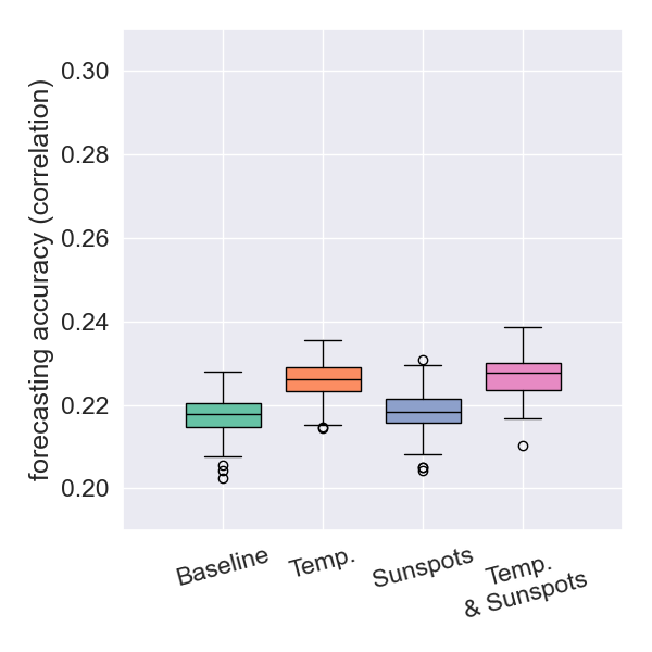any depth

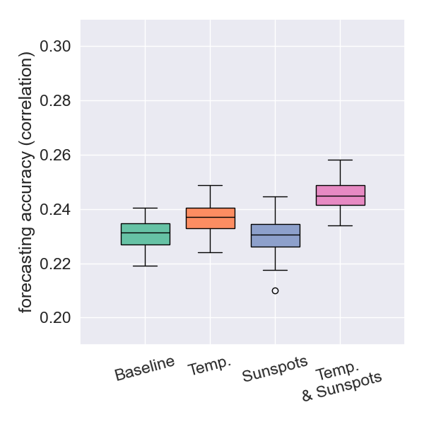depth < 100km

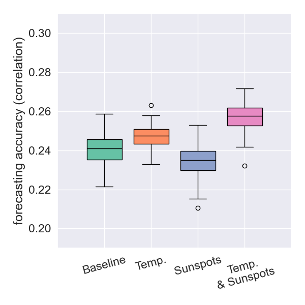depth < 50km

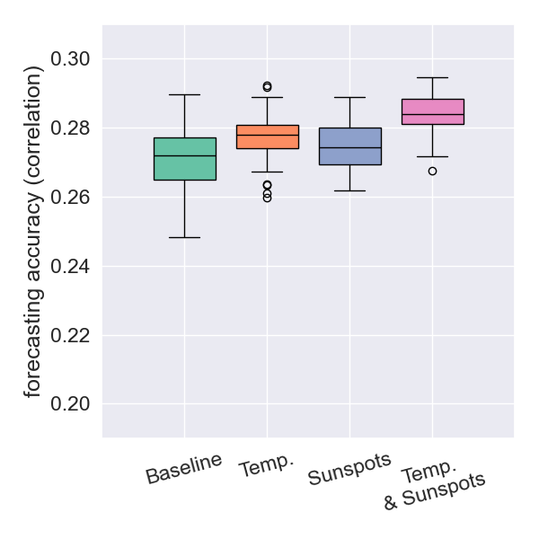depth < 30km

• The results strengthen the idea of a causal connection between surface temperatures and earthquake magnitudes.
• The incremental improvement from using both datasets is modest, indicating informational redundancy.
• This redundancy suggests that the Sun influences earthquakes via the same thermal pathway by which it drives surface temperatures.

Forecasting Results: Balkans

• The inclusion of sunspots overall provided better improvements than surface temperatures.
• The highest correlation for this region was achieved when both sunspot and temperature data were used in conjunction.
• The biggest improvements were observed when restricting the dataset to shallow earthquakes

any depth

depth < 100km

depth < 50km

depth < 30km

• The results strengthen the idea of a causal connection between surface temperatures and earthquake magnitudes.
• The incremental improvement from using both datasets is modest, indicating informational redundancy.
• This redundancy suggests that the Sun influences earthquakes via the same thermal pathway by which it drives surface temperatures.

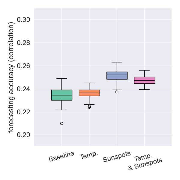
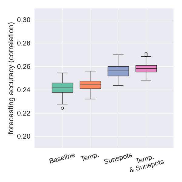
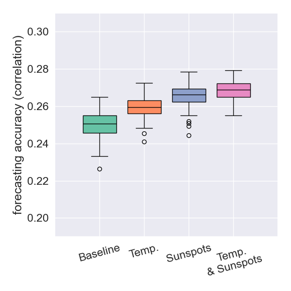
Forecasting Results: New Zealand

• Using temperature data yields a correlation that is not statistically different from the baseline.
• Using sunspot data results in a significantly better correlation.
• The importance of temperature data becomes more pronounced as earthquake depths are restricted to be shallower.

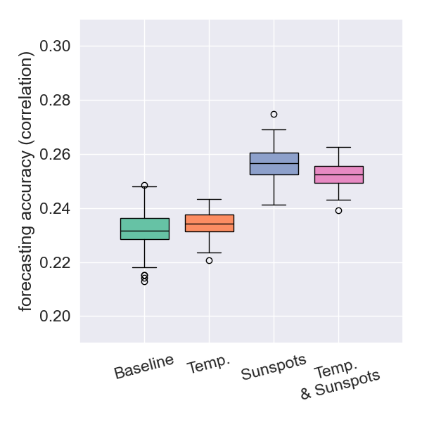any depth

depth < 100km

depth < 50km

depth < 30km

• The results strengthen the idea of a causal connection between surface temperatures and earthquake magnitudes.
• The incremental improvement from using both datasets is modest, indicating informational redundancy.
• This redundancy suggests that the Sun influences earthquakes via the same thermal pathway by which it drives surface temperatures.

Variations Depending on Earthquake Depth

• Many natural phenomena that influence earthquakes (ice melt, sea-level changes, storms) primarily exert their effects at shallow depths.
• These phenomena are often linked to atmospheric temperature and sunspot activity.
• Idea: If temperature and/or sunspots influence earthquakes, the intensity of this effect should vary with earthquake depth.

Analyzing the Evidence

• The idea that atmospheric temperature affects earthquakes is accepted, but is the influence significant or negligible? Our results provide insights.

Ongoing Research: Neural Networks in Earthquake Forecasting

• We have extensively analyzed the applications of edit distances.
  • Edit distances allow us to extract a very particular kind of information from earthquakes.
• How can we concilliate our results with what is in the literature (e.g. statistical indicators)?

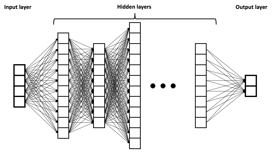
• Neural Networks are flexible tools that could help us achieve that.
• However, a common trend is to progressively increase model size and depth, hoping greater capacity yields better performance.

A Problematic Tendency

• From a Statistical Learning Theory (SLT) perspective, this is an issue.luxburg2011statistical
• Expanding a network's architecture increases its capacity (e.g., VC dimension), heightening the risk of overfitting.vapnik1998statistical
• The common response is regularization (dropout, early stopping, etc.).
• However, this is not a complete solution for seismic forecasting:
  • With limited and noisy data, even well-regularized large models can produce unstable results.
  • Heavy regularization on oversized models can be difficult to interpret.

The Core Problem in Statistical Learning Theory (Opt.)

• The goal of a learner is to find a function \(f\) that minimizes the true risk (generalization error): \[ R(f) = \mathbb{E}_{(x,y)\sim\mathcal{D}}\big[\,\ell(f(x),y)\,\big] \]
• However, we can only minimize the empirical risk on our training sample \(S\): \[ \hat{R}_n(f) = \frac{1}{n}\sum_{i=1}^n \ell(f(x_i),y_i) \]
• Central Question of SLT: Under what conditions does a small empirical risk imply a small true risk?

• The answer depends on the space of admissible functions \(\mathcal{F}\) (the set of all possible models the learner can choose from).
• The generalization gap is bounded by the complexity, or capacity of \(\mathcal{F}\): \[ \big|R(f) - \hat R_n(f)\big| \le \mathcal{N}(\text{capacity of } \mathcal{F}, n) \]
• A larger, more complex \(\mathcal{F}\) increases the risk of overfitting.

The Importance of Capacity Control (Opt.)

• This leads to the classic bias-variance trade-off:
  • If \(\mathcal{F}\) is too small (low capacity): high bias (model can't capture the underlying pattern).
  • If \(\mathcal{F}\) is too large (high capacity): high variance (model fits noise in the training data).
• The key is to precisely control \(\mathcal{F}\) so it's small enough to prevent overfitting, but large enough to contain the function we're looking for.
• Two Strategies for Capacity Control:
  1. Directly restrict the space \(\mathcal{F}\): Our primary approach. Design a smaller, dedicated architecture (e.g., fewer parameters, constrained connectivity).
  2. Regularization: Penalize complexity while searching in a larger space (e.g., \(\ell_1, \ell_2\), dropout, early stopping). A complementary, but less direct, technique.
• Our Argument: Many ML approaches for earthquake forecasting use unnecessarily large \(\mathcal{F}\) and rely only on regularization.

Space of Admissible Functions: $\mathcal{F}$ (Opt.)

A Capacity-Aware NN Architecture

• Motivated by SLT, we designed a custom neural network with deliberately reduced capacity.
• How? By constraining the first layer to be not fully connected, we reduce the space of admissible functions \(\mathcal{F}\) without sacrificing expressiveness.
• Instead of starting with a large model and taming it, we design models whose capacity is constrained to reflect our domain knowledge.
• Core Innovations:
  1. Calculating seismicity indicator features over various time-window lengths (short-term and long-term).
  2. Inclusion of edit distances and seismicity indicators in the same prediction framework
  3. A hierarchical neural network where the first layer has dedicated subnetworks for each time-window length.

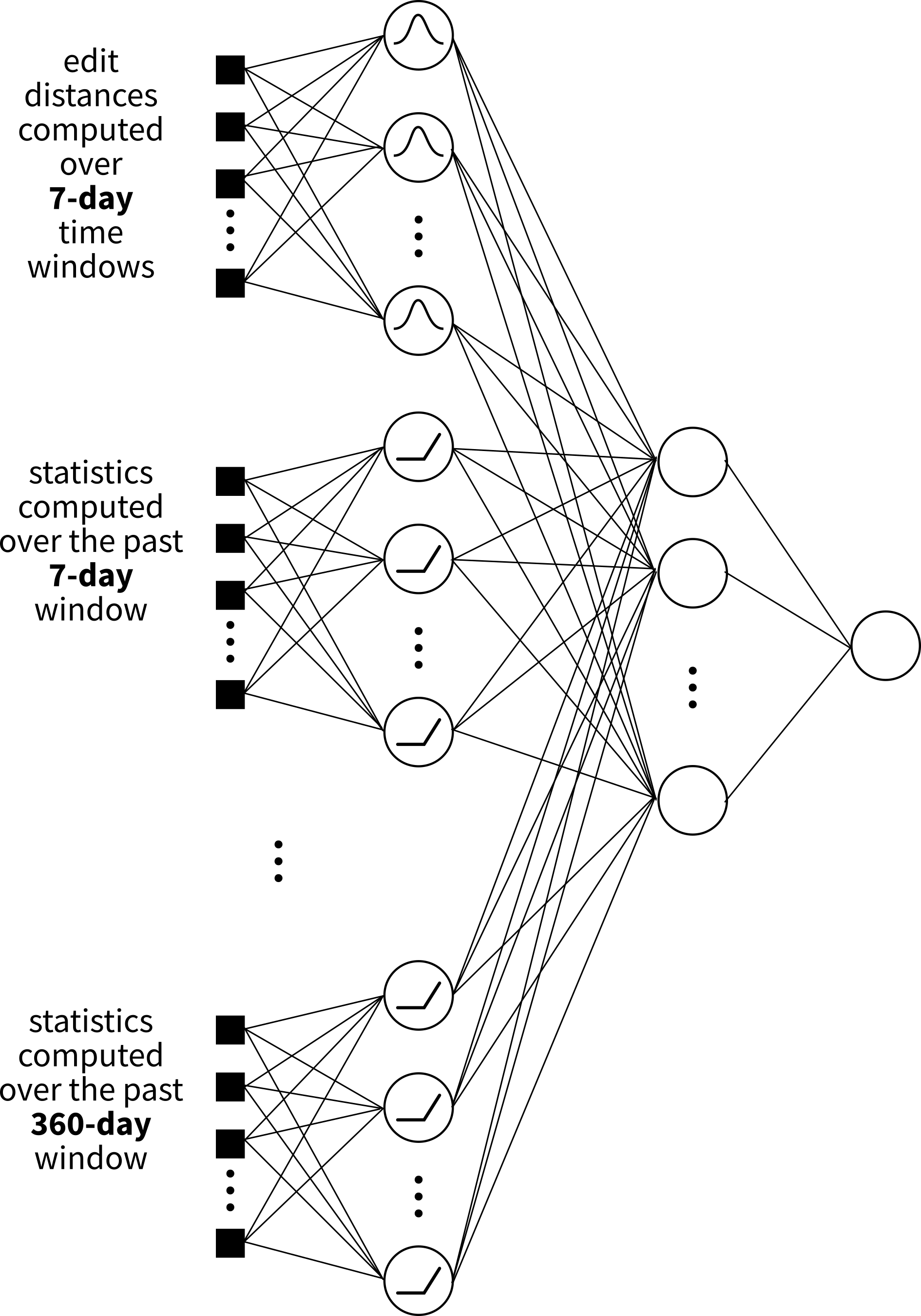
Hierarchical Architecture & Features

Seismicity Indicators (per window):

• T-value
• Mean magnitude
• Rate of sqrt-seismic energy
• Time since first large event
• Gutenberg-Richter slope & intercept
• GR fit error
• Magnitude deficit
• Coefficient of variation of inter-event times

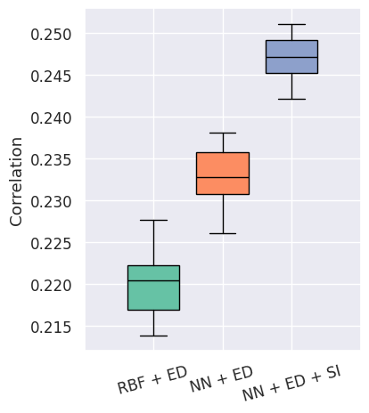
Preliminary Results

• Applied to catalogs from New Zealand, Japan, and the Balkans.
• Average improvement in forecasting accuracy:
  • ~11.8% vs. radial basis functions.
  • ~10.6% vs. NN with only edit distances.
• The model is in its early stages and shows great promise for future improvement.

Japan Prediction Results

Application to Interregional Seismic Interactions

• The proposed neural network was then used to analyze interregional seismic interactions.
• The literature provides strong evidence that distant seismic regions are interconnected through both statistical correlations and physical triggering mechanisms.
• Large-Scale Stress Transmission & Correlation:
  • Tenenbaum et al.tenenbaum2012earthquake reveals strong correlations between regions in Japan over 1000 km apart.
  • Correlations also exist between seismicity at different depths in distinct areas.takayama1992correlation

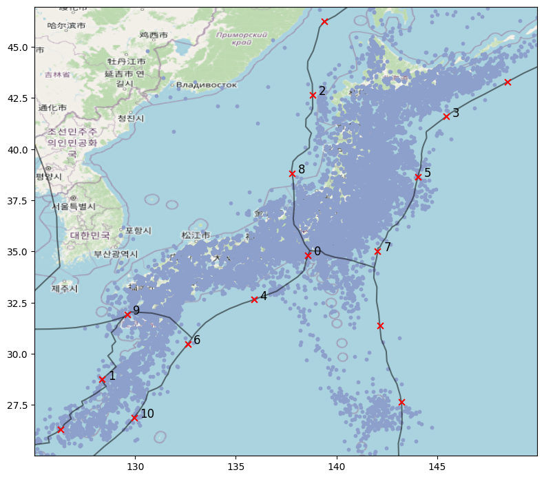
Methodology

• To analyze causal links, Japan and New Zealand were divided into subregions based on centroids over tectonic plate boundaries.
• Three Experimental Settings:
  1. Cross-region nowcasting: Data from region A to predict current max magnitudes in region B.
  2. Cross-region forecasting: Data from A to predict future max magnitudes in B.
  3. Joint-region forecasting: Data from A + B to predict future max magnitudes in B.

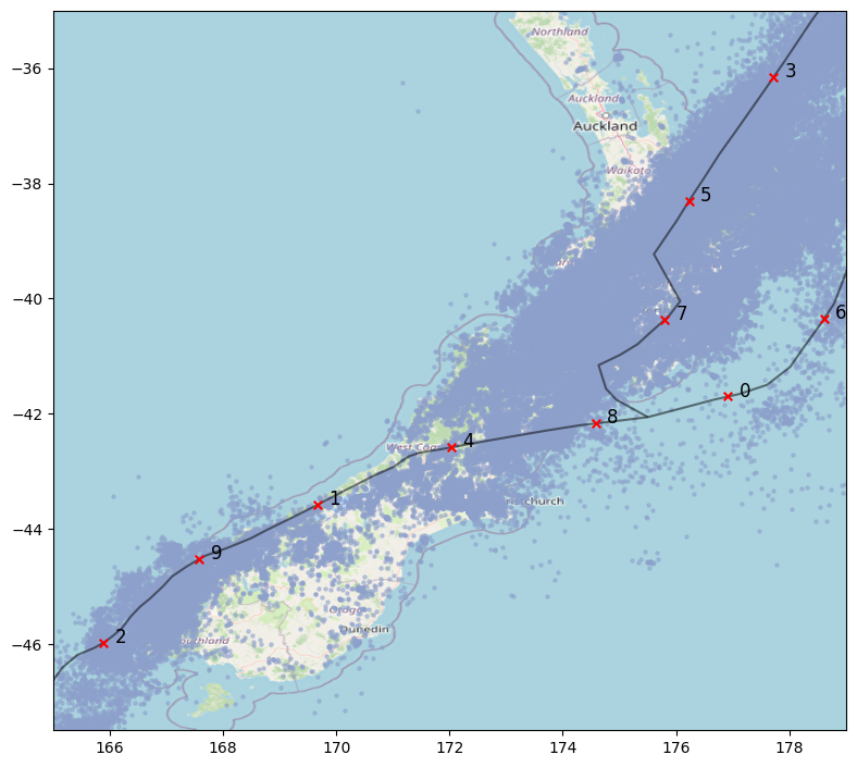
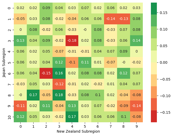
Cross-Region Nowcasting Results

• We see mixed positive and negative correlations, but the average was statistically positive in both directions (JP → NZ and NZ → JP).
• For example, predictions for NZ subregion 1 (Lake Pearson) showed a clear positive correlation.

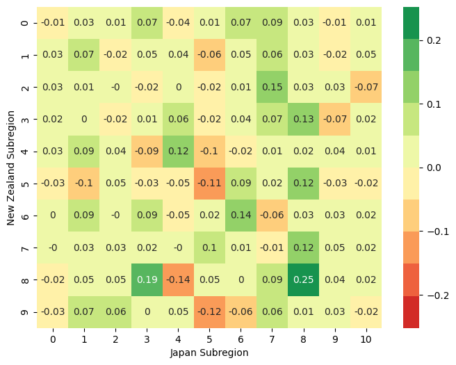
Forecasting & Joint-Region Results

• Cross-Region Forecasting:
  • Observed a positive average correlation when using JP data to predict for NZ, and vice-versa.
  • Example: NZ subregions 7 (Whanganui) & 8 (Wellington) helped forecast for JP subregion 8 (Nagaoka).
• Joint-Region Forecasting:
  • On average, adding data from the distant region did not improve local forecasting accuracy.
  • However, some NZ subregions (2, 7, 8) did benefit significantly from JP earthquake data.
  • Thus, the information brought by including data from another region could be in some sense redundant.
• Interpretation: The connection suggests the earthquake generating processes in both regions might share a common driving force.
• The lack of improvement could also be due to limitations of the current model, warranting further investigation.

Thesis Contributions: A Multi-faceted Analysis of Edit Distances

• This thesis analyzes the use of edit distances in earthquake forecasting from several novel perspectives:
• Efficient Computation:
  • Streamlined edit distance calculation, leveraging parallel computing to make the analysis of large seismic datasets feasible.
• Theoretical Grounding (during my master's):
  • Formulated the forecasting problem on a solid theoretical basis, using Huke's embedding theorem to justify time-windows and edit distance as a natural metric between them.

Thesis Contributions: A Multi-faceted Analysis of Edit Distances

• Dynamical Systems Perspective:
  • Conducted a deep analysis of the coupling between earthquakes and other dynamical systems (the Sun and Moon).
  • Results indicate a link between lunar tides to seismicity, with a strong correlation between differential pulls & earthquake magnitudes.
  • Provided strong evidence for a thermal pathway linking solar activity to seismicity, improving forecast accuracy.
• Bridging Methodologies:
  • Pioneered the integration of our edit distance framework with what is most often used in the literature: statistical indicators.
  • This is done by proposing a novel hierarchical neural network architecture.

Overall Conclusion & Future Outlook

• This work establishes edit distance as a powerful, theoretically-grounded, and computationally feasible tool for earthquake forecasting.
• Future Directions (this semester):
  • Development and refinement of the hierarchical neural network to effectively combine diverse precursor data.
    • Inclusion of other statistical indicators.
    • Testing other types of layers (e.g. RNNs, attention layers).
  • Completion of the joint-region analyses, including the Balkan region.

Thank You!